Generating Synthetic Images of Marine Plastic Using Adversarial Networks
Gautam Tata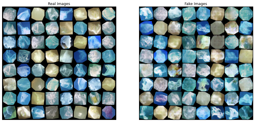
Background
Marine plastic pollution poses significant ecological threats. Automated detection and cleanup methods using computer vision and deep learning have shown promise, but are limited by the scarcity of training datasets. Our research explores using Generative Adversarial Networks (GANs) to produce synthetic images of marine plastic, addressing this data shortage.
Reading Resources: Our Paper on Using CV and DL to detect Epipelagic plastic, The University Of Minnesota’s paper on general-purpose marine debris detecting algorithm, and The Ocean Cleanup’s paper on floating plastic detection on rivers.
The primary issue for this approach is regarding the availability of datasets to train the computer vision models. The JAMSTEC-JEDI dataset is a good collection of Marine Debris off the coast of Japan on the seafloor. However, apart from this dataset, there is a vast discrepancy in the availability of datasets. For this reason, I have utilized the help of Generative Adversarial Networks, The DCGAN in particular, to curate synthetic datasets that could theoretically be a close replica of real datasets over time.
GAN and DCGAN
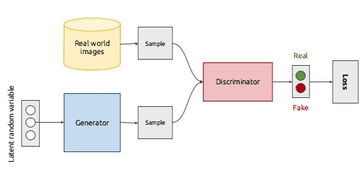
GANs, or Generative Adversarial Networks, were proposed by Ian Goodfellow et al. in 2014. GANs consist of two simple components called Generators and Discriminators. An oversimplification of the process is as follows: The Generator's role is to generate new data, and the Discriminator's role is to distinguish between the generated data and the actual data. In the ideal scenario, the Discriminator cannot distinguish between the generated and real data, resulting in ideal synthetic data points.
DCGAN is a direct extension of the GAN architecture mentioned above, except it uses Deep Convolutional Layers in the Discriminator and generator, respectively. It was first described by Radford et al. in the paper Unsupervised Representation Learning With Deep Convolutional Generative Adversarial Networks. The Discriminator consists of strided convolutional layers, while the generator consists of convolutional transpose layers.
PyTorch Implementation
In this method, we are going to be applying the DCGAN architecture on the DeepTrash dataset ( Citation Link: https://zenodo.org/record/5562940#.YZa9Er3MI-R, Released under the Creative Commons Attribution 4.0 International license). To become more familiar with the DeepTrash dataset, consider reading my paper A Robotic Approach Towards Quantifying Epipelagic Bound Plastic Using Deep Visual Models. DeepTrash is a collection of plastic images in the epipelagic and abyssopelagic layers of the ocean curated for marine plastic detection using computer vision.
THE CODE
Installing Requirements
We install all the basic requirements for building our GAN models, such as Matplotlib and NumPy. We will also utilize all the tools (such as neural networks and transformations) from Pytorch:
from __future__ import print_function
#%matplotlib inline
import argparse
import os
import random
import torch
import torch.nn as nn
import torch.nn.parallel
import torch.backends.cudnn as cudnn
import torch.optim as optim
import torch.utils.data
import torchvision.datasets as dset
import torchvision.transforms as transforms
import torchvision.utils as vutils
import numpy as np
import matplotlib.pyplot as plt
import matplotlib.animation as animation
from IPython.display import HTML

# Set random seem for reproducibility

manualSeed = 999
#manualSeed = random.randint(1, 10000) # use if you want new results
print("Random Seed: ", manualSeed)
random.seed(manualSeed)
torch.manual_seed(manualSeed)
Initializing our Hyperparameters
This step is relatively straightforward. We will set up the hyperparameters we want to train the Neural Network. These hyperparameters are borrowed from the paper and PyTorch’s training tutorial on training GANs.
# Root directory for dataset
dataroot = "/content/pgan"

# Number of workers for dataloader
workers = 4
# Batch size during training
batch_size = 128

# Spatial size of training images. All images will be resized to this
#   size using a transformer.
image_size = 64

# Number of channels in the training images. For color images, this is 3
nc = 3

# Size of z latent vector (i.e., size of generator input)
nz = 100

# Size of feature maps in generator
ngf = 64

# Size of feature maps in Discriminator
ndf = 64

# Number of training epochs
num_epochs = 300

# Learning rate for optimizers
lr = 0.0002

# Beta1 hyperparam for Adam optimizers
beta1 = 0.5

# Number of GPUs available. Use 0 for CPU mode.
ngpu = 1
Generator and Discriminator Architectures
Now, we define the architectures for the generator and Discriminator.
# Generator
class Generator(nn.Module):
    def __init__(self, ngpu):
        super(Generator, self).__init__()
        self.ngpu = ngpu
        self.main = nn.Sequential(
            nn.ConvTranspose2d( nz, ngf * 8, 4, 1, 0, bias=False),
            nn.BatchNorm2d(ngf * 8),
            nn.ReLU(True),
            nn.ConvTranspose2d(ngf * 8, ngf * 4, 4, 2, 1, bias=False),
            nn.BatchNorm2d(ngf * 4),
            nn.ReLU(True),
            nn.ConvTranspose2d( ngf * 4, ngf * 2, 4, 2, 1, bias=False),
            nn.BatchNorm2d(ngf * 2),
            nn.ReLU(True),
            nn.ConvTranspose2d( ngf * 2, nc, 4, 2, 1, bias=False),
            nn.Tanh()
        )

    def forward(self, input):
        return self.main(input)

        # Discriminator
class Discriminator(nn.Module):
    def __init__(self, ngpu):
        super(Discriminator, self).__init__()
        self.ngpu = ngpu
        self.main = nn.Sequential(
            nn.Conv2d(nc, ndf, 4, 2, 1, bias=False),
            nn.LeakyReLU(0.2, inplace=True),
            nn.Conv2d(ndf, ndf * 2, 4, 2, 1, bias=False),
            nn.BatchNorm2d(ndf * 2),
            nn.LeakyReLU(0.2, inplace=True),
            nn.Conv2d(ndf * 2, ndf * 4, 4, 2, 1, bias=False),
            nn.BatchNorm2d(ndf * 4),
            nn.LeakyReLU(0.2, inplace=True),
            nn.Conv2d(ndf * 4, 1, 4, 1, 0, bias=False),
            nn.Sigmoid()
        )

    def forward(self, input):
        return self.main(input)
Defining the Training Function
After defining the Generator and Discriminator classes, we define the training function. The training function uses the generator, Discriminator, optimization functions, and the number of epochs as the arguments. We train the generator and Discriminator by recursively calling the train function until the required epochs. We do this by iterating through the dataloader, updating the Discriminator with new images from the generator, and calculating and updating the loss function.
def train(args, gen, disc, device, dataloader, optimizerG, optimizerD, criterion, epoch, iters):
  gen.train()
  disc.train()
  img_list = []
  fixed_noise = torch.randn(64, config.nz, 1, 1, device=device)

  # Establish convention for real and fake labels during training (with label smoothing)
  real_label = 0.9
  fake_label = 0.1
  for i, data in enumerate(dataloader, 0):

      #*****
      # Update Discriminator
      #*****
      ## Train with all-real batch
      disc.zero_grad()
      # Format batch
      real_cpu = data[0].to(device)
      b_size = real_cpu.size(0)
      label = torch.full((b_size,), real_label, device=device)
      # Forward pass real batch through D
      output = disc(real_cpu).view(-1)
      # Calculate loss on all-real batch
      errD_real = criterion(output, label)
      # Calculate gradients for D in the backward pass
      errD_real.backward()
      D_x = output.mean().item()

      ## Train with all-fake batch
      # Generate a batch of latent vectors
      noise = torch.randn(b_size, config.nz, 1, 1, device=device)
      # Generate fake image batch with G
      fake = gen(noise)
      label.fill_(fake_label)
      # Classify all fake batches with D
      output = disc(fake.detach()).view(-1)
      # Calculate D's loss on the all-fake batch
      errD_fake = criterion(output, label)
      # Calculate the gradients for this batch
      errD_fake.backward()
      D_G_z1 = output.mean().item()
      # Add the gradients from the all-real and all-fake batches
      errD = errD_real + errD_fake
      # Update D
      optimizerD.step()

      #*****
      # Update Generator
      #*****
      gen.zero_grad()
      label.fill_(real_label)  # fake labels are real for generator cost
      # Since we just updated D, perform another forward pass of the all-fake batch through D
      output = disc(fake).view(-1)
      # Calculate G's loss based on this output
      errG = criterion(output, label)
      # Calculate gradients for G
      errG.backward()
      D_G_z2 = output.mean().item()
      # Update G
      optimizerG.step()

      # Output training stats
      if i % 50 == 0:
          print('[%d/%d][%d/%d]\tLoss_D: %.4f\tLoss_G: %.4f\tD(x): %.4f\tD(G(z)): %.4f / %.4f'
                % (epoch, args.epochs, i, len(dataloader),
                    errD.item(), errG.item(), D_x, D_G_z1, D_G_z2))
          wandb.log({
              "Gen Loss": errG.item(),
              "Disc Loss": errD.item()})

      # Check how the generator is doing by saving G's output on fixed_noise
      if (iters % 500 == 0) or ((epoch == args.epochs-1) and (i == len(dataloader)-1)):
          with torch.no_grad():
              fake = gen(fixed_noise).detach().cpu()
          img_list.append(wandb.Image(vutils.make_grid(fake, padding=2, normalize=True)))
          wandb.log({
              "Generated Images": img_list})
      iters += 1
Monitoring and Training the DCGAN
After establishing the Generator, Discriminator, and Train functions, the final step is to call the train function for the number of epochs we defined.
#hide-collapse
wandb.watch_called = False
# WandB – Config is a variable that holds and saves hyperparameters and inputs
config = wandb.config          # Initialize config
config.batch_size = batch_size
config.epochs = num_epochs
config.lr = lr
config.beta1 = beta1
config.nz = nz
config.no_cuda = False
config.seed = manualSeed # random seed (default: 42)
config.log_interval = 10 # how many batches to wait before logging training status

def main():
    use_cuda = not config.no_cuda and torch.cuda.is_available()
    device = torch.device("cuda" if use_cuda else "cpu")
    kwargs = {'num_workers': 1, 'pin_memory': True} if use_cuda else {}

    # Set random seeds and deterministic pytorch for reproducibility
    random.seed(config.seed)       # python random seed
    torch.manual_seed(config.seed) # pytorch random seed
    np.random.seed(config.seed) # numpy random seed
    torch.backends.cudnn.deterministic = True

    # Load the dataset
    transform = transforms.Compose(
        [transforms.ToTensor(),
        transforms.Normalize((0.5, 0.5, 0.5), (0.5, 0.5, 0.5))])

    trainset = datasets.CIFAR10(root='./data', train=True,
                                            download=True, transform=transform)
    trainloader = torch.utils.data.DataLoader(trainset, batch_size=config.batch_size,
                                              shuffle=True, num_workers=workers)

    # Create the generator
    netG = Generator(ngpu).to(device)

    # Handle multi-gpu if desired
    if (device.type == 'cuda') and (ngpu > 1):
        netG = nn.DataParallel(netG, list(range(ngpu)))

    # Apply the weights_init function to randomly initialize all weights
    #  to mean=0, stdev=0.2.
    netG.apply(weights_init)

    # Create the Discriminator
    netD = Discriminator(ngpu).to(device)

    # Handle multi-gpu if desired
    if (device.type == 'cuda') and (ngpu > 1):
        netD = nn.DataParallel(netD, list(range(ngpu)))

    # Apply the weights_init function to randomly initialize all weights
    #  to mean=0, stdev=0.2.
    netD.apply(weights_init)

    # Initialize BCELoss function
    criterion = nn.BCELoss()

    # Setup Adam optimizers for both G and D
    optimizerD = optim.Adam(netD.parameters(), lr=config.lr, betas=(config.beta1, 0.999))
    optimizerG = optim.Adam(netG.parameters(), lr=config.lr, betas=(config.beta1, 0.999))

    # WandB – wandb.watch() automatically fetches all layer dimensions, gradients, and model parameters and logs them automatically to your dashboard.
    # Using log="all" log histograms of parameter values and gradients
    wandb.watch(netG, log="all")
    wandb.watch(netD, log="all")
    iters = 0
    for epoch in range(1, config.epochs + 1):
        train(config, netG, netD, device, trainloader, optimizerG, optimizerD, criterion, epoch, iters)

    torch.save(netG.state_dict(), "model.h5")
    wandb.save('model.h5')

if __name__ == '__main__':
    main()
Results
We plot the loss incurred by the generator and discrimination during training.
plt.figure(figsize=(10,5))
plt.title("Generator and Discriminator Loss During Training")
plt.plot(G_losses,label="G")
plt.plot(D_losses,label="D")
plt.xlabel("iterations")
plt.ylabel("Loss")
plt.legend()
plt.show()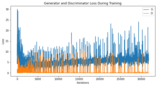
We can also pull up an animation of how the generator generated images to see the difference between the real and the fake images.
#%%capture
fig = plt.figure(figsize=(8,8))
plt.axis("off")
ims = [[plt.imshow(np.transpose(i,(1,2,0)), animated=True)] for i in img_list]
ani = animation.ArtistAnimation(fig, ims, interval=1000, repeat_delay=1000, blit=True)

HTML(ani.to_jshtml())
CONCLUSION
In this article, we discussed the use of Deep Convolution Generative Adversarial Networks to generate synthetic images of marine plastic that researchers can use to extend their current marine plastic dataset, allowing researchers to extend their dataset with a mix of real and synthetic images. The adversarial network still needs much work. The ocean is a complex environment with varying illumination, turbidity, blur, etc. However, this is a theoretical starting point that other researchers can build on. If you want to improve the results and build a better network architecture, please contact me at gautamtata.blog@gmail.com.